JBioPro
Updated on April 23, 2004. The most actual version can be accessed here.
Move planets with your brainwaves
Signal parameters on element level
Processing and initialization order
Feedback and comment is welcome
JBioPro is a deployment tool that should help with analyzing signals in real time. Primarily goal is to use it with EEG, ECG, EMG, GSR, EOG and other bio-feedback devices, but generally any type of input/output processing is possible. All functionality is contained in processing components; no assumption on the nature of processing was made in system core. Visual designer tool is provided to optimize preparation of analyze. JBioPro name stands for Bio-Processor or Body-Input-Output-Processor. Development was done primarily in Java. Originally JBioPro was designed to run on PDA, but it works also and even better on PC.
I am professional software developer and I started thinking about something like JBioPro even before I discovered the OpenEEG project. On the beginning, because of my long experience with software development, I wasn’t that eager, I knew how easy it is to start something and then loose interest. Unfortunately I did not find any tool, which would fully fit my needs. I started development in about March 2003. Initially it was just command line software running on PDA linux, later I started adding more functionality to use it on PC. I do not know if JBioPro will have any relevant use, but I have used it for quite a while and I like it. The decision to make it public is quite recent, I though that maybe it would be useful for biofeedback community. The reason I hesitated so long was because it required considerable effort to make is usable for users without programming experience, and I did not even know if anyone would like it. I also did not want to present something partially done to avoid disappointment just on start.
There is still much to do, software development is almost like never ending story, but at least it is possible now to perform quite advanced analysis. And it is relatively easy to build extensions.
JBioPro is a tool that should allow anyone to get easily from an idea to reality. A good idea is the most important and there are many people that are very interested in that subject and have good ideas, but do not have possibility to introduce them. Hopefully JBioPro and other tools will make it possible.
I think that human-to-machine interfaces have great potential, but not that much popularity yet. There are a few subjects that should be doable already now, but it is not that obvious how to do that with 100% certainty for example:
· how to recognize that someone is sleeping and measure the level of sleep,
· how to recognize REM (rapid eyes movement),
· how to recognize that someone is relaxed,
· how to measure levels of relaxation so that we know where to aim,
· how to measure dynamics and effectiveness of entrainment, and others.
There are already many theories, research and observations about the above for example with using combinations of alpha, beta waves etc., but not that many proved implementations. There are many cases, many factors, dependencies, various types of bio feedbacks and few concrete prescriptions of how to do this in practice and together (for example ECG together with EEG during jogging). Maybe JBioPro will help with that by giving option to exchange working designs and verifying them by different people.
I have been developing JBioPro according to my analyzing needs, so everything that exists now was used in my private research.
1. Main goal during designing JBioPro was to make it flexible, extendible and simple to use (to prepare analyzing design quickly). It is not easy to combine all those features together and perhaps there will many significant changes in future.
2. I focused on features not on appearance, so at this moment graphics is rather basic.
3. Another important factor during designing was highest possible performance of processing. Java is not the best in that so it was even more important. At this moment I can say honestly that performance is very decent. In future if better is needed, the processor can be optimized or even rewritten from scratch in C.
4. I created JBioPro so that it can be useful in real life research and to know better how the brain/mind works. It is not my goal to do software development just for the sake of doing it, without real necessity. Therefore any propositions for new features will be carefully considered, unless something is very easy or you offer a donation.
Usually JBioPro works as a real time processor of data arriving from biofeedback device. However if you do not have any device compatible with JBioPro, you can try first use it with one of the archive files or connect it to someone else’s device via network (with Neuroserver or JBioPro network elements). To read JBioPro archive files (bpa), use FileStorageSource element.
So far I have used JBioPro primarily with my ModularEEG, therefore there are many notes related to that EEG device in this manual, but JBioPro is designed to work with anything else.
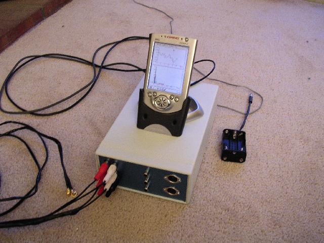
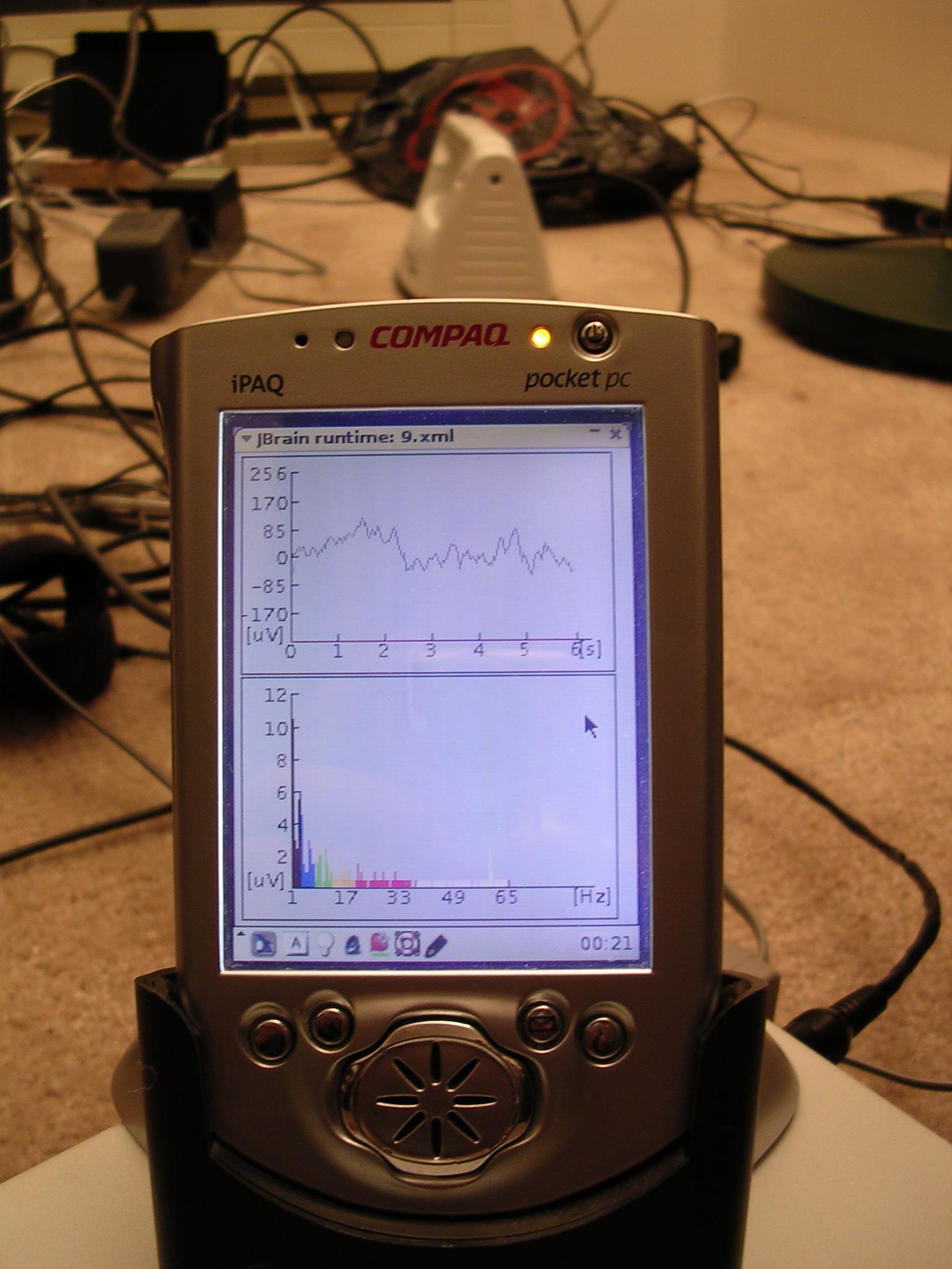
Initially JBioPro was designed to work on PDA (see picture). I believe PDA is great opportunity, the devices are already very powerful (comparable to PC from before a few years) and they will be faster. Portability is great asset.
Recently I have used JBioPro only on PC, since version 1.0 it has never been run on PDA with graphics. This is because it is much easier to do conduct research on PC, and JBioPro’s designs are still in research phase. I want to come back to PDA as soon as there are concrete stable designs, which do not need further experimentation.
Installation process is very easy:
1. Install java runtime environment (JRE) version 1.4.2 or higher. Here is information about older java versions. If you already have java on you PC, then you can skip this step. To check whether java is already installed type in command line: “java –version” (without quotes); if your version is later or equal to 1.4.2, then you are ready to go. Otherwise go to this page http://java.sun.com/j2se/1.4.2/download.html and download JRE for you operating system and install it (installation process is straightforward).
2. Unzip jbiopro-install-XX.zip to the directory you want to have it installed, for example c:\jbiopro.
3. To start JBioPro in command line go (with cd command) to jbiopro folder, and type: start.bat (on Windows) or start.sh (on UNIX, Linux). After that you should see JBioPro graphic user interface window. If no graphic appears, type start_console.bat and read the messages.
JBioPro is platform independent, it should work on any machine with java virtual machine including Windows, UNIX, Linux, MAC and PDA systems.
Since it is supposed to work on PDAs (Personal Digital Assistant) with limited resources therefore it requires not much processing power. I would say that any machine that runs java 1.4 should be ok. Probably Pentium II with 64M RAM is minimum, I did not try it on anything else then my PC though. The faster the machine the smoother processing will be, especially with graphic display.
JBioPro was developed and tested mostly on Windows XP machine with P4 2.4GHz processor and 512M RAM. In the earlier stage of JBioPro (was named JBrain at that time) it was tested on PDA Linux (www.handhelds.com); here and here are pictures of my PDA showing real time FFT processing of the EEG signal. I also have RedHat Linux available.
Installation on PDA may be more difficult because of compatibility issues.
1. Find JVM for your PDA operating system. You need to determine if you need graphic display, it may be much easier to run it first only as command line. I successfully installed and run java with graphic on Blackdown JRE 1.3.1 on Familiar Linux.
2. Check if your JVM supports:
a. AWT (if graphic is used)
b. Serial port access
c. MIDI and sounds (if sound feedback is used)
d. External shell command execution (e.g. for external sound player)
3. Now you can continue with JBioPro installation as described above.
4. Consider using external C objects for time consuming operations, e.g. FFT.
Potential issues I encountered:
· Performance was low for serial port with P2 protocol due to poor serial port support in OS. That is why I implemented new protocol v21 for ModularEEG. This may be heavily dependent on PDA and how serial port data transmission is done in operating system.
· I could not run external process from Java on Blackdown JRE (to play sounds with external sound player); it finally worked with C extension object.
At this stage the best way to upgrade is to install new version and copy files (designs, archives etc) to appropriate folder in new jbiopro installation directory. In future it is possible that an option for migration between versions will be implemented.
JBioPro is already quite powerful when it comes to processing capabilities; it has over 40 processing elements plus over 20 functions at this moment. The most important feature is however that addition of new elements is very easy. New elements can be implemented in java even without advanced programming skills or C language (FFT was implemented that way as an example). Other technologies like jpython should be also possible.
Some of the features:
1. Read and decode stream from ModularEEG device with P2 or v21 protocols, all channels included.
2. Show results graphically in real time (oscilloscope, vectors, 2D color vectors, bars, orbits, numbers and others) with carefully scaled values (microvolt, digital, percent).
3. Processing on streams or vectors.
4. Scalar transforms (average, min, max, range mapping, range filtering, rate controlling and others).
5. Vector transforms (average, RMS, min, max, sub-vectors, power split).
6. Various conversions across vector and scalar (FFT with windowing etc).
7. Save/read data stream in/from file(s).
8. Send/receive data stream to/from network sockets.
9. Send/receive data stream to/from raw file (can be useful for example if ModularEEG data was stored earlier in file or if serial port is a file).
10.Store data in wav format so that it can be read and analyzed with using regular sound editors.
11.Store data in a format that can be imported (and analyzed) in Excel type software or database.
12.Various signal source simulators.
13.Sound feedback (midi, wav files or using external player like mp3).
14.Multiplexers, mixers, debuggers, mappers, counters, timers etc.
15.Pattern recognizers (experimental, not yet implemented).
Some of the above names may not be compliant with common naming convention used in biofeedback field. Please let me know if some other names would more appropriate.
At this moment JBioPro supports only ModularEEG device http://sourceforge.net/projects/openeeg. I have only this one. Architecture is however open not only for any other devices, but also for connecting to several different devices simultaneously. To add support for a new device you can either build new JBioPro element for that, or send it to me together with protocol specification, and I will do that.
User interface is now rather simple, main effort was put on features and flexibility. In the main mode there are 2 windows: designer and runtime. Designer window serves mostly as a design editor, and runtime shows the processing outcome.
Designs are created and edited with mouse and keyboard.
Brief description:
· To add new element press right mouse button and choose “new” from the popup menu. Choose any element from the list.
· To edit existing element highlight it and then press right mouse button over it and choose “properties” or press “space” on keyboard.
· To move existing element to new position press left button and drag.
· To resize existing element press and drag on the small triangle in the bottom right corner.
· To learn about functionality press right mouse button and choose “description”.
· To add connection between output and input of two elements, click on small rectangle inside the element, then move mouse to destination and click again.
· To remove an element or a connection, highlight it and choose “remove” with right mouse button or press “Del” button on the keyboard.
· To view a problem in the element (this can be observed when a small red cross appears in the bottom left corner of the element), choose “view error” with right mouse button.
· To load previously saved design, choose from menu System->load and choose design file.
· To save your design in file, choose from menu System->save as.
· To switch between edit and view mode of Runtime, choose Runtime->set edit mode (Runtime->set view mode) in Designer menu.
· To highlight group of elements press Ctrl button while clicking next elements.
Validation of the properties values in elements in not yet fully done. This means, that it can happen now that a wrong value will cause unexpected behavior or even cause an element to cease working. This will be improved gradually in time.
Runtime window can work in 2 modes: view or edit. Either mode can be chosen in designer window’s menu. The first mode is basically for setting layout of the display charts. The viewing mode is set by default when JBioPro starts.
Below there are a few example designs that demonstrates some capabilities of JBioPro. Those designs should be considered as a start points for analyses rather then ready to use solutions. More designs that were not included with installation bundle can be found here.
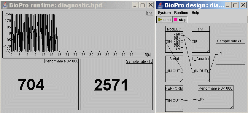
This is good bio-design for a start or to verify system configuration. See example picture. The default version is configured to work with ModularEEG, but anything can be connected as a source (network connection, simulator etc.).
It gives some information that can be helpful:
1) Check if serial device is sending any data.
a) If a signal appears on the oscilloscope, then it indicates the device (ModularEEG) and serial port are likely ok.
b) If nothing appears, then the configuration and setup should be checked again.
2) Check the performance of the system and JVM.
a)
In the Performance
0-1000 window there is numeric value that represents how our system and JVM
(Java Virtual Machine) performs. This picture
shows results from Windows XP, P4 2.66Hz machine. The higher the value, the
better performance. Value 1000 is max that in reality can never be reached. If your
value is below 10 then this indicates that performance is probably too low to
run JBioPro (this is up to personal judgment).
You need to wait for at least 10 seconds after processing started to get proper
value from this window.
b) Performance is dependent on the number of elements in a design. There are two elements needed to measure current performance: P_Counter and Performance 0- 1000. They can be put inside any other design to check performance there. Usually it is enough to measure it only here.
3) Check the sample rate of the input device.
a)
In the Sample
rate x10 window a sample rate of the input source (ModularEEG, simulator etc.)
is displayed. The actual rate is multiplied here by 10 (result is measured within
the last 10 seconds). In case of ModularEEG this value should be about 2560.
This value may fluctuate and be not always very precise, it depends on the
overall system performance and how other elements in the same design behave,
but it should show a value close to the above.
You need to wait for at least 10 seconds after processing started to get right
value from this window.
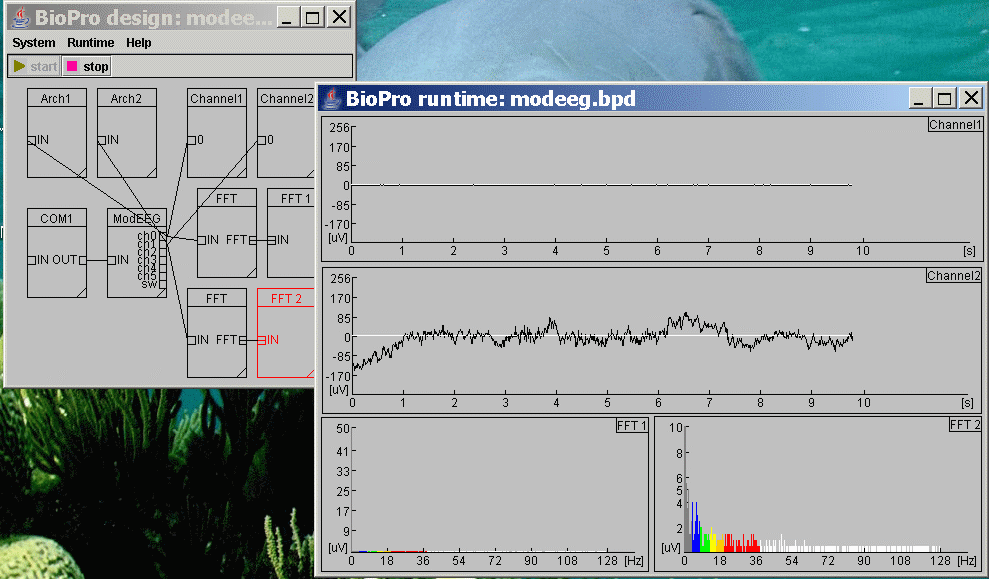
This design gives ability to display both channels from ModularEEG device. It can be modified for the number of channels or further extended. This design is also a good start point to verify that ModularEEG works with JBioPro. See picture.
This design shows FFT capabilities available at this moment. This includes FFT transformation, operations on vectors and scalars, display 1D, bar 1D and 2D charts. See picture. The 2D display was created quite recently and had not yet occasion to be really used in analyses, however it seems to have some potential.
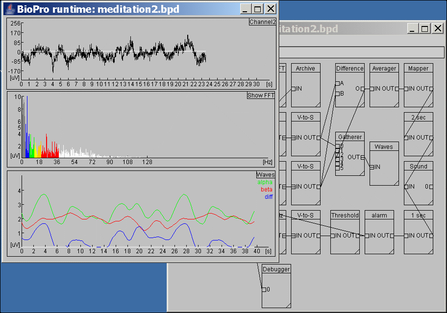
This design should help with meditation practices. See the picture. At this moment it simply measures amplitude of alpha waves and a sound is played (every 2 seconds) that represents the measured value. The higher alpha the higher is the sound pitch. All parameters can be modified to meet specific needs. For example instead of taking MAX from brain waves vectors, perhaps RMS would be better. The sounds pitch order can be changed so that for higher difference lower sound is played.
This design can be a good start point for other more specific trainings.
This is extended version of the alpha training design. See picture. It contains additional feedback control prepared specifically for checking skin-electrode connection. I found it useful with my active electrodes to make sure that the connection is stable. If connection is weak, linear signal often goes behind the range and exactly that is being checked here. Additionally 60Hz interference level is being checked, if it goes above threshold level, it also may indicate weak connection.
This may be especially useful if we want to try that with eyes closed, or when graphic display is not available or not easy (like with PDAs). Together with PDA this design gives elegant solution for portable meditation devices.
Here is short description of the fields in the above design:
This design provides ability to record EEG during the night. See design picture and example results. Besides recording it also generates sound feedback (alarm) when electrode-skin connection is too weak. The electrode-skin connection is being checked against:
1. 50-60Hz mains hum
2. Signal out of range
3. Flat signal
The first two tests are like in meditation design, the last one is useful with active electrodes; they tend to behave like that (flat signal) sometimes.
Additionally this design contains delayed sound feedback; it means that the alarm is not played for the first 20 minutes of sleep, or during any time when there is proper response for at least 90% during last 20 minutes (being checked every second). This feature is important with dry active electrodes, which are sensitive to even small movements.
The design attached to JBioPro installation bundle contains network server (SServer on diagram), it is prepared to work with PDA as proxy. It can be replaced with SerialPortDevice element the same way as in previous designs.
There are 2 designs coming with JBioPro that use OrbitalDisplay element. See picture1 and picture2. First is only for single brainwave, and the other for three different brainwaves. Planets move around their center (Sun). Their speed depends on brainwave amplitude. The goal is to control the movement. It is possible to set threshold for each planet which determines direction it should move.
It is probably better to try first the orbital1.bpd design. You may want to set those parameters first:
· brainwaves frequency range (in “Band” element)
· Planet movement threshold (in “Orbit” element). The threshold can be set for example to value that appears on digital numeric chart (it shows current amplitude of the brainwave). That way planet will move slowly, right or left. The goal may be to make it still, or moving.
· If the rotation is too fast (or too slow), you can either change the Threshold (the speed depends on difference between brainwave amplitude and the threshold), or Velocity (in “Orbit” element).
· Averaging function can be set in “V-to-S” element. To achieve the best effect here use RMS or MAX function.
· To change FFT response time, modify Period field (in “FFT_T” element). The longer is this period, the smoother are the movement changes.
The orbital2.bpd design works the same as the above, but there are three different brainwaves that can be trained in the same time.
This section shows example biofeedback results done with JBioPro that might be worth of further research.
Here are links to other sites that published interesting results with JBioPro:
· http://www.georgs-home.com/gallery/eeg
Here is my first nightly recording I did with using JBioPro. See the picture. Dry active electrodes were placed on forehead. This location is probably the reason why signal goes behind the default range of ModularEEG scale sometimes. My first guess is that should be REM (Rapid Eyes Movement). But this can be also any other movement, I noticed that active electrodes are quite sensitive to any movements of the skin (like wrinkling). Maybe I will try recording on other spots, but it is not easy because of hair and also my sleeping habits.
Anyway, the results are quite good to me. It is noticeable that the theta waves went much above alpha sometimes. That indicates being in sleep (?). I am not sure about the delta. How much the muscles interfere here? The delta is very high, but it is always like that when electrodes are on forehead and I did noticed, that it is not like that on back of the head (I verified that with pin active electrodes once).
This session was recorded between 11pm and about 1:30am. The horizontal scales on the pictures are in seconds. There are two charts with the same result but different ranges to allow viewing the full range and also more details simultaneously.
I think that the times between 3726-4968 and 7000-end indicates some uneasy dreams (I do not remember anything). I do remember that at about 1:30 I woke up because of something unpleasant. I believe much of that was caused by the headband with electrodes I had on my head, I am still not used to it.
· It is proven and reliable technology, used for instance by NASA on Mars :-).
· It is the easiest and the most popular solution for portability. We want JBioPro running on PDAs, and we may not want to create designs there.
· Java development is very effective when it comes to searching for bugs.
· Although the performance of Java is lower then C language, with JIT (Just in Time) virtual machine, the speed is reasonable in most cases. If higher performance is needed it can be easily optimized with using C through JNI extension.
· External C libraries (like numerical recipes) can be reused and included easily with JNI interface.
· If properly done, then the same code does run on many different systems without any modifications. This can depend heavily on JVM (Java Virtual Machine) chosen, it is recommended to use Sun’s JVM whenever possible. Although they are not always the fastest, they provide relatively consistent environment.
· Java is perfect for elegant object oriented development that can be easily extended.
JBioPro relays on the following external libraries:
JBioPro is supposed to work on various operating systems, including those with limited resources like PDAs or even cell phones. That is one of the reasons why Java was chosen as primary language, extensions in C language are possible and easy for performance increase whenever required.
· Visual runtime part of JBioPro is done with pure AWT since it is fast and most portable. Visual designer was originally done in AWT, but now was converted to Swing.
· Whenever possible processing operations are done with using only integer variables (no floats or doubles), because coprocessor availability can not be assumed.
· Threads are not recommended.
JBioPro was tested mostly on Windows XP, some tests were done on PDA Linux and RedHat linux. It should run without any issues on any brand Linux or UNIX system. It should also run on Mac (if there is a JRE with Java 1.3) and others.
Design is strictly object oriented. Configuration and design files are stored in xml format for flexibility and scalability. There is no restriction e.g. for a number of elements in JBioPro, limits are set only by hardware resources.
There are 3 main modes how JBioPro can be executed:
· Full mode, both visual designer and runtime windows are shown.
· Visual Runtime mode, only runtime window is shown. Processing is automatically started when the program starts.
· Command line runtime mode, no graphics is displayed. All components that use graphics are not being processed at all. Processing is automatically started when the program starts. This option can be useful when the graphics is no available, or simply to increase performance.
Usually the design process is done on standalone PC and then the runtime can be executed on other devices (like PDA) with using of the same design file.
System can be used with one bio design at a time. Each design is stored in a single bpd (JBioPro design) file. The same design file is used for either of the three run modes. Basically it is assumed, that the design process is being done on standalone PC and execution process on any system.
Stress has been put for optimal and simple process of adding new functionality to JBioPro. New functionality is stored in elements. Each element must inherit from jbiopro.processing.Element class. A few methods must be provided in each new element:
· process(), this method is executed by main engine sequentially in all elements of the design Therefore it is permitted to operate on non-synchronized buffers since they can’t be modified during that time (unless multithreaded elements are used). This method should be optimized for the highest possible performance. If possible only integer variables should be used. Threads are not recommended. Inside the method you simply take values from input stream array and write the results to output stream.
· reinit(), this method is executed when new design is loaded, or when a modification to an existing element was made
· start(), executed just before processing is started
· stop(), executed as soon as processing is stopped
· getInputCount()/getOutputCount(), returns number of inputs/outputs provided in this element
There are dozens other methods that can be overridden in an element (see Element class); the above are the most basic. Each already existing element can serve as start point for further development.
To add quickly a new element:
1. Copy an existing java element from impl folder or package jbiopro.processing.impl and rename it.
2. Rename the class name inside so that it is identical as your file name and remove (or change if needed) package name.
3. Put your runtime algorithm inside processing() method and initialization inside reinit() method. See how this is done in other elements from that package.
4. Make public all properties (class fields) that you want to be editable from GUI (user interface). Internal variables should be not public.
5. Compile .java file to .class file, and copy class file to the jbiopro/impl folder. More information about compilation is here.
6. After JBioPro restart you should see your element name in the list of available new elements.
I created an example HelloWorld element. It is available here.
1. To see if it works, just copy HelloWorld.class file to jbiopro/impl folder. After JBioPro is restarted, it should be visible in the GUI list of new elements. Try to add it in the designer window.
2. If the above worked then remove the previous HelloWorld.class file, then copy HelloWorld.java to jbiopro/impl folder and follow steps provided in the below compilation chapter.
3. If all the above worked, then you are ready to create your element. You can simply edit the HelloWorld.java source. Or copy it to another file (remember, that the class name (inside the file) must match file name (.java).
The default JBioPro installation procedure includes only JRE (Java Runtime Environment) that is good to run JBioPro, but not enough to compile anything. To compile new Element (or whole JBioPro package) you need Java SDK. If you plan to make compilations, instead of JRE you better download and install J2EE SDK (it includes JRE). It can be downloaded from http://java.sun.com/j2ee/1.4/download.html.
To compile new jbiopro Element go to jbiopro/impl directory (assuming there is YourFile.java file) and type in command line:
javac -classpath ../ext/jbiopro.jar YourFile.java
After successful compilation file YourFile.class should appear in the same folder. It will be available in elements list after JBioPro is restarted.
Pipes represent data flow channels. At this moment there are two types of pipes: raw streams and vector streams. Raw stream value (up to 32 bit) can be considered as a vector with just one element, but optimized for higher performance.
There are input pipes and output pipes. One output pipe can be connected to many input pipes. Input pipe should be connected to only one output pipe. If input is connected to many outputs then it works as multiplexer, but without known order. Each input pipe has an internal buffer.
Aside from traditional stream conversions, JBioPro introduces new way of data processing. In JBioPro it is possible to process vector stream and that option gives new possibilities comparing to traditional stream filters. In conventional applications, input stream is being filtered with various types of digital filters. For example to get the amplitude of alpha brainwave a bandwidth filter is applied on the signal and the amplitude of the filtered result is measured.
In JBioPro new way of processing is possible. Signal can be first converted to vector (for example with FFT transformation or any other), and then all further processing can be done on vectors. One of the reasons to something like that was for performance increase (many filters can be slower then single FFT). Another reason is that each filter introduces some level on distortion to the input signal, while vector processing operates on the same values.
Of course traditional filtering is still possible with no restrictions. Hopefully someone with more experience with filters (I do not have any) will add some to JBioPro.
At this moment only 1-dimensional vector streams are available. Higher dimensions are possible in this architecture but not likely to be implemented any time soon.
As was stated before, filter functionality can substituted with FFT and vector processing. Example of how to recognize alpha wave was provided in this design. It is possible, that filters will be added later to JBioPro. If someone is interested, let me know. From version 1.0.3 it is possible to set very short time response in FFTTransform element e.g. 0.25 or 0.125 s.
Information about signal parameters like rate, range or number of bits is provided on element level (as oppose to global level). An element can get these values from other element connected to one of its inputs. An element can also modify its own values if necessarily. For example if an FFT transformation is being done 4 times per second, then it means that the rate is now 4, and it should return this value when asked for the rate.
Each element’s properties must be standardized so that the system can recognize them properly. All public properties of the element are automatically saved (and retrieved) in design files. Therefore new element does not need to provide its own way of storage.
In the visual designer window, public fields of each element can be viewed with mouse and edited. This applies to both static and non-static properties.
It is possible to customize description that is being shown in visual designer for each individual property.
All internal temporary properties in the element should never be public.
Java has built in JNI interface that allows additions of C-based coding, which can fully cooperate with all java components. This technology is already used in JBioPro, for example current FFT transformation can run as java or C. There are at least two reasons to do something like that (use C extensions): it can increase processing performance (especially without JIT java) and it also allows reuse of existing C libraries.
JBioPro should work with any java version starting from 1.3.1. Almost all development was done in 1.2.2; the only exception in this moment is media support (MIDI and internal wav player). So it should work on 1.2.2 without sounds or with external sound library or player. Final testing was done on 1.4.2 and this version is recommended and supported.
There are many different versions of Java for PDAs. And there are also a few operating systems (most popular are probably Windows CE, Zaurus and Familiar linux). There are JRE versions that work only on one platform and sometimes only on some models of PDA. Therefore it is not easy to choose which one is the best.
I installed familiar Linux on my Ipaq 3765, and I use now Blackdown 1.3.1 JRE for ARM processor. Both can be downloaded from www.handhelds.org. Although this JRE is rather slow, at least it has been so far quite compatible with regular java JRE on PC.
But it took me considerable time to learn and configure everything, especially Java graphics was difficult.
This released version of JBioPro has never run on PDA (earlier versions did), since I use my PDA now as a network proxy, it only pass data between PC and ModularEEG through wireless network.
This configuration file contains global settings for JBioPro. Currently it is used to store information about elements. All permanent settings will be here eventually.
Whenever it is easy signal amplitude from input device is scaled in microvolt. The idea was to make microvolt a common measurement unit independent from a device. There are also other scales: digital and percentage. There are 6 possible amplitude scales available in JBioPro:
· microvolt or uV – microvolt values starting from 0 and more
· digital or digi – digital values starting from 0 and more
· percent or % – percent values from 0 to 100
·
balanced microvolt or =uV – balanced microvolt
values, any range is possible
(although usually they will be within max range)
·
balanced digital or =digi – balanced digital
values, any range is possible
(although usually they will be within max range)
· balanced percent or =% – balanced percent values from -100 to 100
For each balanced value, the 0 value means the middle of the whole range. For example if in ModularEEG, the digital value is from 0 to 1023, the digital balanced 0 will equal 512 of unbalanced digital value.
At this moment most eeg devices operate on microvolt (or fraction of microvolt). Other biofeedback devices (like EMG or ECG) may use values of higher amplitudes.
Digital scale represents direct integer values being received from biofeedback device. In case of ModularEEG, the output range is now from 0 to 1023, and this corresponds to range from -256 micro-volts to +256 micro-volts on balanced micro-volt scale. JBioPro operated now on 32 bit numbers; therefore any device with up to 32 bit sample length can be supported.
Percentage scale is relative to full range allowed in an element. So the 50% means half of full possible range.
Not implemented yet.
Time scales are at this moment shown in seconds only. Eventually more units will be provided. Now they are relative (since the recording started), eventually they will also show absolute time.
Each element can specify, whether its predecessor (another element connected to one of its inputs) must be initialized earlier. Most elements do that (see the source code). Because of that, sometimes it is not possible to connect elements in a loop. Fortunately this problem doesn’t occur very often, since not all elements require first initialization of its predecessor.
Elements are being processed in the same order as they were initialized.
JBioPro graphics is now very simple but also quite powerful. It should run on all platforms since there is no machine specific code. It is possible to build more advanced features (like 3D display), but that would require more advanced graphics tools (that utilize system dependent libraries like DirectX). It can be done, since java provides support for 3D graphics, question is how useful this can be.
JBioPro installation package includes all necessary
drivers to access serial port on Windows. On Linux it is possible to read from
serial port device like from file (e.g. /dev/ttyS0) and therefore driver is not
required, however you have to set port parameters (baud, parity etc.) manually
with using linux tools. It is also possible to install driver on Linux; the
advantage is that all parameters of the serial port could be then set in JBioPro.
Sun doesn’t provide driver for Linux now, but there are other implementations
e.g. http://www.geeksville.com/~kevinh/linuxcomm.html.
For further information about serial port installation or problems with serial
port access see Sun’s site: http://java.sun.com/products/javacomm/downloads/index.html.
JBioPro can be started without any options, and that will be full runtime with designer and default (last loaded) design. Command line options can alter its behavior. Command line syntax:
java jbiopro.Main [filename.bpd] <-or|-op> <-diagnostic> <-log filename> <-start> <-root folder_path> <-logs folder_path>
Where:
· -or: only runtime window is shown, and processing is started automatically after start.
· -op: only processing is started automatically after start
· -diagnostic: set diagnostic mode (debugging messages printed on console). Additional menu with diagnostic options are available with this option.
· -log <filename>: all text messages are written to this file (and console)
· -start: processing is started automatically after start (useful only when working with visual Designer)
· -root <folder_path>: path to JBioPro folder, should be provided if started from different folder.
· -impl <folder_path>: path to folder with elements implementations, default is jbiopro/impl.
· -logs <folder_path>: path to folder where logs are stored, default is jbiopro/logs.
In some elements it is possible to specify colors. At this moment only those predefined colors are available (case sensitive): black blue cyan darkGray gray green lightGray magenta orange pink red white yellow. In future more options (RGB and other scales) can be provided if needed.
Very often it is necessarily to average results in order to make them smoother (ScalarTransform, VectorTransform, VectorSingleTransform) or to show on chart as a single line (VectorToScalar). Therefore it is important to understand how different averaging functions work. Here are example charts that show a few averaging functions on the same input signal:
· JTF signal of delta (1-4Hz), FFT on 512 points (2 seconds with 256Hz input)
· JTF signal of delta (1-4Hz), FFT on 1024 points (4 seconds with 256Hz input) – this result comes from the same input signal, but has 2 seconds delay when comparing to the above.
It shows graphic vertical bar.
This element works the same way as Mixer, but the input signal is mixed with constant integer value. Although the value in the field is being entered as float, it is automatically converted to digital value with regards to the chosen scale.
This object counts number of occurrences. Other functions will be added in future (e.g. rising edges, falling edges).
· Time period [s] – if greater then 0, then occurrences are counted within this time period; otherwise they are counted since processing started. Real time is measured; it is independent from input rate.
· Count – functions:
o SAMPLES – counts incoming samples
o INVOCATION – counts how many times the processed() method was invoked.
This is diagnostic element; it prints all incoming values on console. This element is hidden by default. To make it available uncomment its section in jbiopro/config/configuration.xml file.
Stream values are saved in a text file; digital values are separated with semicolons.
This object performs FFT transformation and sends vectors as results.
· Period [s] – processing time interval, this must be power of 2, for example 1, 2, 4, 8, 16 etc. or 0.5, 0.25, 0.125, 0.0625 etc. Make sure the input rate is high enough for very small periods.
· Rate – how many computations is done per second.
· Fast response – if this is set, then all data in input buffer is being processed according to above rate, otherwise only the most recently received data is processed once and the buffer is purged.
· Subtract bias – removes bias from the result.
· Maximum frequency – shows maximum frequency calculated according to the above settings.
· Frequency resolution – shows the frequency precision.
· FFT type – chooses FFT algorithm. At this moment there are 3 types:
1. INTEGER – performs calculations on integers. It is the fastest method but can process samples of only up to 15 bits.
2. FLOAT - performs calculations on floats, this option is slower then INTEGER (about 2 times slower on my PC). The main advantage is that it always works, for example INTEGER may not work well for input samples of more then 15bits.
3. NATIVE – allows use of external (native) FFT. The library must be connected to JBioPro with JNI interface.
· Window – provides options for FFT windowing type.
· High resolution of amplitude – if set, then FFT output resolution is increased to 15 bits. This means that in some other elements (that process FFT results) digital scales or values may not work any more (unless defined for 15 bit values). The microvolt and percentage scales are fine.
Reads data from file stored earlier with FileStorageWriter object.
· filePath – file name and path to read. If this file doesn’t exist, then the most recent file is loaded whose name begins with this path; this can be useful when option makeUniqueNames was chosen in FileStorageWriter element.
· readInLoop – if this is set then, after all data is read, reading from beginning of the file is continued.
· keepOriginalRate – If this is set, then data is read from file with the same rate as stored, otherwise all data is read up to available space in buffers.
· keepOriginalTime – if set then original time will be set to mainProcessingTime variable. The time is calculated either by rate or by time markers written by FileStorageWriter.
· readChunk – if greater then 0, then this number of bytes is read from archive (and written to output) at a time. Otherwise the number is equal to half of the available space in output buffer.
· Loaded file – this field shows the name o the archive file. This can be useful, when the latest file is being loaded automatically (by date of creation). This option can’t be modified, it is only for information. To change the loaded file - modify filePath.
· Start time [s] – if greater then 0, then this elements starts reading from this time point (relatively to archive begin), otherwise this option is ignored. If this option is set, then it will be automatically reflected in all Oscilloscope and VectorLineDisplay charts of the same design.
· End time [s] – if greater then 0, then this element stops reading at this time point (relatively to archive begin), otherwise this option is ignored. If this option is set, then it will be automatically reflected in all StreamDisplay and VectorLineDisplay charts of the same design.
This object saves data in file in JBioPro proprietary format.
· filePath – file name and path to save
· appendExisting – if this is set, then the data is appended to the file, otherwise file is overwritten
· makeUniqueNames – if this is set, then each new session is saved in new file with unique name. To retrieve the data (with using FileStorageSource) user needs to know which file to read (see file names in the same folder as the original file).
· Time marker period [ms] – if this is greater then 0, then time markers are written along with data in the archive file periodically (period defined here in milliseconds); they can be later used to find precise time when something was archived. This option is especially useful when the rate of the input is variable. This will be also needed for recording precisely response to a short stimulation.
At this moment, this element saves 16bit data bytes only. In future it will be improved to give ability to save up to 32bit data samples (number of bits will be chosen automatically depending on device’s capability). It is also possible that some compression will be added.
This element performs various conversions on one channel data format. JBioPro internally operates on 4-byte signed integers. Sometimes it is required to convert this to different format, for instance during communication with another software (via network or while reading a file).
Fields:
· adjustRange – if this is set, then the range is shifted to the center of the destination range.
Functions:
· TO 2 Unsigned Little-Endian
· TO 3 Unsigned Little-Endian
· TO 4 Unsigned Little-Endian
· FROM 2 Unsigned Little-Endian
· FROM 3 Unsigned Little-Endian
· FROM 4 Unsigned Little-Endian
· TO 2 Signed Little-Endian - PCM
· TO 3 Signed Little-Endian
· TO 4 Signed Little-Endian
· FROM 2 Signed Little-Endian – PCM
· FROM 3 Signed Little-Endian
· FROM 4 Signed Little-Endian
This object is used as a sound feedback. Each input value is played as a different note. Appropriate range mapping is usually necessarily to fit into desired sound pitch. Notes values can be 0-127, so the mapping should use a sub-range of that. Value 60 represents note C.
Fields:
· velocity – determines the midi sound velocity (see MIDI specification on www.midi.org for further details)
· restartSound – if set, then sound is restarted for each new input value, if not set, then sound is restarted only if input value is different then previous one.
· midiDevice – any available in system midi device can be used.
· instrument – it is possible to choose instrument only for Default Synthesizer midi device.
This object performs various operations on two input streams; both input streams should have the same rate. The rate of the output is the same as the rate of the input A (unless ONLY_INPUT_B option was selected).
Balanced option means, that the input stream is supposed to be balanced (the zero value is in the middle of the whole range).
Functions:
1. SUM, BALANCED_SUM is A + B
2. DIFFERENCE, BALANCED_DIFFERENCE is A - B
3. MULTIPLICATION, BALANCED_MULTIPLICATION is A * B
4. AVERAGE (A + B) / 2
5. MAX is max(A, B)
6. MIN is min(A, B)
7. ONLY_INPUT_A, ONLY_INPUT_B this option can work as a selector between inputs.
This object decodes P2 protocol stream from ModularEEG, details can be found on http://openeeg.sourceforge.net.
This object decodes v21 protocol stream from ModularEEG (details on http://www.geocities.com/jfolt/bw/modeeg_firmware/index.html). This protocol is useful whenever higher performance or backward communication is required. On PC, P2 protocol is usually good enough.
First all buffered samples from input 1 is written to output, then all from input 2, end so on. This element is especially useful if order (priority) is important. Otherwise the same functionality can be achieved when the same input is connected to many outputs.
This object connects to a specified network server, and once a connection is established it exchanges scalar data through network.
Fields:
· Host – address of the server, can be DNS or IP address.
· Port – port to connect to.
This object listens on a port (in thread), and once a connection is established it exchanges data through network. Only one client can be connected at a time.
Fields:
· Port – port number the server listens to.
This element can be used to read data from NeuroServer. Only one data channel can be read here at a time. To read more then one channel, add more elements and choose different channels.
Fields:
· Receive channel – determines which channel to read. Default is 0.
· deviceNumber – if this value is less then 0, then the first found NeuroServer EEG device is chosen automatically. Otherwise a device with this number is chosen.
This element can be used to write data to NeuroServer. Only one data channel can be written a time. This channel can be then read by other NeuroServer clients.
This object displays current value from the input as a number or text.
This is unique and powerful element. Planets move around their center (Sun). Each planet’s movement speed is based on biofeedback value. Number of planets is configurable. Planets icons are configurable, so it is possible that other pictures are used e.g. cars or train or anything else. It can be used in various ways for example:
1. Train your desired brainwave or try to control specified brainwave. Set Rotation threshold so that planet moves right or left depending on amplitude of the brainwave.
2. Show each wave band as a different planet. The higher is the brainwave amplitude the faster is planet’s velocity. The lower is the frequency of the wave the farther the planet from the center or vice versa etc.
3. Train for just one specific wave. When desired wave amplitude increases and reaches higher level, next planets starts to move. First the planet in the center and last the planet on the far orbit. The goal is to keep moving all planets.
4. Set threshold to desired value and try to switch rotation from one direction to another.
5. Play a race game with other people (as many as you want) connected either to the same computer or via network (with NeuroServer or JBioPro network elements). Different planets (or other icons) can represent different people. This can be a start point for other games based on biofeedback.
Fields:
· Planet size – set the size of the planet. Size can be 16, 32 or 64 (pixels). In case of included with JBioPro planets, the size means actual icon width, but in reality this can be any width. Important part is, that the icon file name must be started with one of these numbers (see file names in jbiopro/images folder, for instance: 16_earth.gif).
· Rotation threshold – planet movement depends on this threshold. If biofeedback value is greater then threshold, then planets movement speed is proportional to difference between value and the threshold. If the value is below the threshold, planet moves in other direction. If you want to move the planet only one direction, set this threshold to 0.
· Clockwise rotation – set the planets’ default rotation direction. If marked and if the value is greater then Rotation Threshold, then the planet will move clockwise around the center.
· Show trajectory – show orbital lines for each planet.
· Planet icons – graphic icon files can be specified here, trajectory of each orbit is calculated on base on icon’s actual size.
Shows input stream on graphic chart like on oscilloscope.
Fields:
· Time range [s] – time range in seconds
· Amplitude range [uV] – value range in micro-volts
· Higher precision (lower performance) – if set then all values are printed on screen. Otherwise only 1/N value is printed, when N depends on screen resolution.
· Join points – joins consecutive points drawn on screen.
· Reflect time range – if marked then the time range is set automatically to values provided by any other (predecessor) element that defined them (TimeRangeFilter or ArchiveReaders).
This is an experimental object, it is being implemented. It will run execute neural network trained with PatternTrainer.
· IN – samples
· OUT – recognized sample
This is an experimental object, it is being implemented now. The idea is to build an object which will be able to learn and recognize patterns. I have an idea to do this with neural networks. First a series of input samples will be applied to patternInput and the expected results are applied to patternOutput. Then training is done (inside or outside of JBioPro) and if it was successful, then PatternRunner will execute the neural network.
· IN – samples
· OUT – expected pattern result
· EFF – effectiveness (percent) of the trained neural network.
This object controls the range of the samples values. The output rate depends on the values in the input stream, so it can fluctuate. This object can be valuable for example for controlling unexpected (out of range) behavior or as a threshold sensor.
Fields:
· Inclusive – if this is set, then only the values from within defined range constraints are sent to output. Otherwise only those out of range are sent.
· Bands – defines value ranges.
This object converts values from one range to another, for example if input range is 1-9, and output 21-29, then for input value 7, to output will be sent 27. Or if input range is 100-300, and output is 1-5, then for input 150, value 2 will be sent to output, and for input 200, it will be 3.
Fields:
· invertedOrder – modifies order of the output range, in the last example, for input 150, the output would be 4.
This object controls throughput. Rate means how many samples per second will be passed from input to output.
Fields:
· Number of samples defines maximum number of samples that will be passed to output within specified time range.
· Time range [ms] – rate is calculated for this time specified in milliseconds. For example if number of samples is 4, and time range is 1000, then it means max rate is 4. If number of samples is 4, and time range is 500, then the output rate is 8 (samples per second).
· cleanExcessiveData – input values are pilled in input buffer if the predecessor rate is greater then above rate. To avoid buffer overload this checkbox should be set.
Read raw values from a file.
This object writes to a file the raw values (no headers or formatting).
Transformation is performed on single sample. Output rate is the same as input rate.
Functions:
1. INVERTER - output value is inverted (against middle of the scale). For example if input sample value is 2uV, then the output will be -2uV.
2. DIFFERENCE – output value is the difference between current sample and previous input sample.
3. ABS – takes the absolute value of the sample.
4. BALANCED_ABS – takes the balanced absolute value.
5. WITHIN_DEFAULT_RANGE – if sample is out of the default range, then it is converted to max/min allowed value within the range.
This object creates vectors from several scalar inputs. All scalar inputs should have the same rate. The output rate is the same as the lowest of all inputs rates.
There are a few functions available in this object. All transforms keep the output rate the same as input rate. Transform is being performed on input Sample number samples (as oppose to ScalarSingleTransform).
Fields:
· Samples number – the processing is being done on this number of samples in input buffer. If the number of bytes in buffer is lower, then function is performed on available samples until desired amount of samples arrive.
Functions:
6. AVERAGE – output value is averaged over the number of input samples.
7. MAX – output maximum value from the last N of input samples.
8. MIN – output value is the minimum from the last N input samples.
9. PEAK_TO_PEAK – the maximum difference of signal amplitude is written to output.
This object is used to read from a serial port. It can use either java serial communication (on Windows), or read from a file (useful on linux).
This simulation object can provide various signals.
Fields:
· Frequency array [Hz] - contains array of required signals.
· Amplitude array [uV] – contains array of corresponding amplitudes for above signals.
· Signal range [uV] – output signal range
· Phase shift [0-360] – shifts the phase of the output, this can be useful if more simulation sources are used and different phases are needed between them.
· Noise level [uV] – introduces random noise.
· Output sample rate [Hz] – output sample rate.
This object is used to play sounds that are stored as files. Those can be played either with using internal (java) sound player, or external executable player. If the path to the external player is specified, then this external player is run, otherwise internal java player is used.
For each input numeric value, different sound file is played; file names must be numbers (with a sound file extension); for each possible input value a file with that number name must exist in the folder. RangeMapper or RangeFilter can be useful here to play only within the range of existing files.
There is an example folder with sounds in folder media/ding.
This object converts scalar stream into vector stream.
Functions:
1. FRAME – takes N input samples (defined in vectorLength), creates vector and sends it to output. This is done every N sample (defined in period). So the output rate is input_rate/period.
Takes a vector from input, and sends only part of it to output. It still remembers the original values (min and max). Output vector’s resolution is the same as input resolution.
Fields:
· Low frequency [Hz] – minimum physical value of the sub-vector
· High frequency [Hz] – maximum physical value of the sub-vector
· Output vector size – shows the sub-vector’s actual size.
· Start index – shows the start position of the sub-vector in original input vector.
· End index - shows the ending position of the sub-vector in original input vector.
This simulation object’s parameters are set inside the program. This can be used by programmers only. This element is not available by default. To make it available uncomment its section in jbiopro/config/Configuration.xml file.
This simulation object parameters are set inside the program. This can be used by programmers only. This element is not available by default. To make it available uncomment its section in jbiopro/config/Configuration.xml file.
Shows time since processing started. Now it can show seconds only, this will be extended later to milliseconds, triggered time periods etc.
This object can control data flow in time. It passes only data within the time range. The actual number of samples is calculated on base on sample rate, so the predecessor element must provide valid rate of the signal. I have found this feature particularly useful when analyzing pieces of an archived signal.
Fields:
· Start time [s] – if greater then 0, then this elements starts reading from this time point, otherwise this option is ignored. If this option is set, then it will be automatically reflected in all Oscilloscope and VectorLineDisplay charts of the same design.
· End time [s] – if greater then 0, then this element stops reading at this time point, otherwise this option is ignored. If this option is set, then it will be automatically reflected in all Oscilloscope and VectorLineDisplay charts of the same design.
Creates a graphic chart, where another dimension is added with using colors. This can be useful for example to show a vector changing in time.
It shows present vector value on graphic chart.
Prints on chart all fields of the vector, each with different color.
· Time range [s] – show time range
· Amplitude range [uV] – show amplitude range
· Colors – define colors for each field of the vector. If not provided, then default colors are provided
· Agenda descriptions – description for each vector field in agenda can be defined here. If not specified, then indexes (or physical values) are displayed.
· Reflect time range – if marked then the time range is set automatically to values provided by any other (predecessor) element that defined them.
· Physical agenda – has effect only if there is no Agenda Description field. If marked then physical values are displayed, otherwise vector indexes.
This object works like Mixer but for vectors.
This object contains various transformations on single vector. The output rate is always the same as input rate, functions are preformed on one vector only (as oppose to VectorTransform).
Field:
· Left – defines window length on the left (lower) side of the sample (value) according to chosen function.
· Right - defines window width on the right (higher) side of the sample (value) according to chosen function.
Function:
· AVERAGE - each vector field is averaged over its neighbors.
· MAX - each vector field is set to max value over its neighbors.
· MIN - each vector field is set to min value over its neighbors.
· RMS – each vector field is set to Root Mean Squares of all its neighbour fields: sqrt(sum(Sn^2) / N).
This object converts each vector to scalar value according to chosen function. Output rate is the same as input rate.
Function:
1. AVERAGE – calculated average of all vector values.
2. MAX – takes the maximum from all vector values.
3. MIN – takes the minimum from all vector values.
4. MIDDLE_POWER – calculates index of the vector, so that sum of the values below the index is equal to the sum of value above the index.
5. MIDDLE_POWER_2 – calculates index of the vector, so that sum of the square values below the index is equal to the sum of the square values above the index.
6. SUM – sum of all vector fields: sum(Sn)
7. RMS – Root Mean Squares of all vector fields: sqrt(sum(Sn^2) / N).
8. RS – Root of Squares: sqrt(sum(Sn^2))
This object contains various transformations on vector. The output rate is always the same as input rate, however functions are performed on many samples defined in Samples number field (as oppose to VectorSingleTransform, where transformed is only one vector).
Fields:
· Samples number – defines number of samples upon to perform the transform.
Function:
1. AVERAGE – each vector field is averaged over a period of time. Processing is hold until number of samples is available.
2. MAX - each vector field is set to max value over a period of time. Processing is hold until number of samples is available.
3. MIN - each vector field is set to min value over a period of time. Processing is hold until number of samples is available.
It saves scalar stream in file in wav format, so that it can analyzed later with a sound editor.
JBioPro comes with full source code. It can be downloaded from project site. At this moment most of the class method descriptions are not valid, they should not be used for a reference. Comments inside the code are ok. In JBioPro version 1.0.4 release there are about 230 java classes; this means over 1M of source text and over 38 thousand lines.
Reports with bugs or requests for new features can be sent to me. I may not always be available, but will try to fix issues as soon as possible.
If something is obviously wrong, exit JBioPro and start it again with using start_console.bat. See if there is any additional information that could be helpful there. If you want to report a bug or a problem, save text from the console in a file and attach it to the email with problem description.
Any feedbacks or comments are welcome. I would especially appreciate corrections regarding names of the elements, fields and descriptions. I have had no experience with professional medical applications and the vocabulary I used may be sometimes not appropriate or even misleading. Additionally I begun to use English language actively only a few years ago and this is something that still needs improvement too.
New elements can be added relatively easy now. I will be happy to add something that is really needed (just cool may not be enough). For example I though to add 3D display of the vectors (this could be useful for showing FFT changes in time), but I am not really sure if that is that important. If is, then let me know.
Each new version of JBioPro introduces usually new functionality as well as modifications in current elements. At this moment there is no method for migration from older to newer designs. I try to keep compatibility as much as possible. If something has changed significantly there is a note about it. I also try to make sure, that all example designs will work the same way as before.
As I stated, software development is never ending story. Further development will be continued according to this general list (highest priority on top):
· Bugs fixes
· Small improvements
o Add field for an element description
o Arrays edition
· New elements or new features in existing elements
o Time synchronization between elements for stimulations.
· User interface
o Grouping, so that a few elements can be used as one.
o Import/export of single elements, groups or all designs
o More edition options: selecting and moving multiple elements etc.
o Undo/Redo
· More visual information and options in Designer window.
o Ability to show icons/images in elements to make the look different.
o Display additional text messages on elements (?)
o Dynamic display (e.g. reading position from an archive file).
o Ability to create events dynamically.
JBioPro is free to use or redistribute. However my further support and work on JBioPro may depend on how motivated I am to do so. Even a small donation can give me an incentive for further work. Pay me with PayPal.
JBioPro is licensed as GNU GPL.
Copyright © Jarek Foltynski (www.foltynski.net). All rights reserved.